Global Maps on the World Water Situation prepared for the World Water Assessment Programme (WWAP)
For further information see:
WWAP and World Water Development Report
The following maps were prepared by:
Joseph Alcamo, Petra Döll, Martina Flörke, Michael Märker
Contents
| Map 1 | - Long-term average runoff on a global grid |
| Map 2 | - Long-term average water resources according to drainage basins |
| Map 3 | - 90% reliable monthly discharge on a global grid |
| Map 4 | - Water withdrawals according to drainage basins |
| Map 5 | - Per capita water withdrawals by country |
| Map 6 | - Water stress according to drainage basins |
| Map 7 | - Area equipped for irrigation on a global grid |
| Map 8 | - Water withdrawals for irrigation on a global grid |
| Map 9 | - Water withdrawals for manufacturing industries according to drainage basins |
| Map 10 | - Consumptive water use for cooling in thermal power plants |
| Map 11 | - Water withdrawals for cooling in thermal power plants according to drainage basins |
| Map 12 | - Water withdrawals for households according to drainage basins |
| Map 13 | - Internal renewable water resources generated within a country on a per capita basis, circa 1995 [m³/cap/annum] |
| Map 14 | - Percentage of area under severe water stress based on cell-level computations by country |
| Map 15 | - Change in water stress according to drainage basin |
| Map 16 | - Area equipped for irrigation vs total arable land by country |
| Map 17 | - Increase in irrigation requirement in a typical dry year compared to the long-term average on a global grid |
| Map 18 | - Water withdrawals for irrigation as ratio of the total withdrawals according to drainage basins |
| Map 19 | - Combined map showing the drainage basins under medium or high water stress and the water use sector which claims the highest fraction of withdrawals in these drainage basins |
| Map 20 | - Water use in a certain country’s part of a transboundary river basin as ratio of total water use in the basin |
| Map 21 | - Coefficient of variation of annual discharge according to drainage basins |
| Map 22 | - Annual runoff in the 1-in-10 dry year as a ratio of the long-term average annual runoff on a global grid |
| Map 23 | - Water stress in regions around selected mega cities |
| Map 24 | - Dependence of the countries’ water resources on inflow from neighbouring countries: inflow as a ratio of total water availability (internal renewable water resources plus inflow) |
| References |
Map 1. Long-term average runoff on a global grid
This map shows annual average runoff (the difference between precipitation and transpiration/evaporation) on a global grid, with grid cells of ˝ degree latitude by ˝ degree longitude. The time period is the “climate normal” period (1961-90).

Water is a renewable resource because the loss of moisture via transpiration through plants or evaporation from surfaces is continuously returned as precipitation. In all but the driest parts of the earth the gains in moisture exceed losses, and the excess moisture becomes the runoff shown in Map 1. The enormous variation in climate around the earth leads to great spatial variability in this runoff. The amount and form of local precipitation varies tremendously, and varying conditions of surface temperature and humidity greatly affect the local rate of evaporation. Runoff is highest where precipitation is high, and/or where losses due to transpiration/evaporation are on the low side. These areas include Central Africa, the Alpine and Northern regions of Europe, much of India and South/Southeast Asia, the Amazon basin and parts of the east and west coastlines of Latin America, Central America, and the East and Northwest coasts of North America.
backMap 2. Long-term average water resources according to drainage basins
This map shows discharge as runoff accumulated within drainage basins (accounting for evaporation from lakes and wetlands). For the “climate normal” period (1961-90).

Among its other characteristics, water is a transportable substance – and can be transported either naturally through river beds and gulleys, or artificially through culvert and piping systems. For this reason water can be distributed and made available to users at some distance from its source. But most of the runoff generated within a drainage basin is distributed and used within the same basin because the alternative – pumping water over the hills and mountains on its edges – is usually too technically difficult and/or expensive. Waters within a basin are often stored in reservoirs and distributed within a basin by gravity flow. Hence a part of a drainage basin with more runoff can compensate for another part of the basin with less runoff, and the total discharge over drainage basin area is an approximate measure of the water available to the population in the basin. Map 2 depicts the average water resources available in drainage basins each year over the long-run. While the patterns are similar to the runoff map (see Map 1, long-term average runoff) the differences in local runoff are smoothed out because they are summed over the area of a drainage basin. This map sharpens the contrast between adjacent water-rich and water-poor areas. For example, the differences in water availability between northern and southern India, and between northwestern and western North America become more clear.
backMap 3. 90% reliable monthly discharge on a global grid
This map shows the discharge in each grid cell (surface runoff plus groundwater recharge) resulting from the accumulation of runoff (Map 1) as rivers run downstream. This is a statistical estimate of the minimum monthly flow which occurs over 90% of the months during the climate normal period (1961-90).

The variation in climate from place-to-place leads to the variations in runoff and discharge described in Maps 1 and 2. But climate also varies from season-to-season and year-to-year, and this causes large temporal swings in runoff and discharge. In most drainage basins the difference between the highest and lowest monthly discharge is indeed quite large; in temperate regions river discharge is often enormous because of snowmelt in late winter or early spring and very low in late summer or early autumn because of higher evaporation and lower precipitation. Many tropical regions experience enormous peaks in river discharge during the annual monsoon rains and have minimal flow at the end of the dry season. Besides the relatively predictable seasonal variation in climate, there is also the more unpredictable variation between years which lead to periodic “drier than normal” years and low river flows. Because of these variations, the long-term averages shown in Map 1 (long-term average runoff) and in Map 2 (long-term average water resources) are not particularly good indicators of the water resources that can be counted on each year. A better measure is the “90% reliable monthly discharge” which is the minimum discharge expected in all but the driest 10% of the driest months. Standing out in the map of reliable discharge are the great river carriers of the world such as the Amazon in Latin America, the Yangtze in China, and the Congo in Central Africa which drain large areas and dependably provide large volumes of water in all but the driest of years.
backMap 4. Water withdrawals according to drainage basins
This map shows annual total water withdrawals estimated for 1995 on a drainage basin basis.

Society withdraws large volumes of water each year from the world’s reservoirs, rivers, aquifers and other freshwater and saltwater sources. Major water users are households, factories, power plants and irrigation projects (see Maps 8, 9, 11, 12 on water withdrawals by sector). In Map 4 we show the sum of all withdrawals on a drainage basin basis. The units of the map [mm/a] indicate how much water is withdrawn per unit area of a drainage basin. High water withdrawals occur as expected in densely populated areas such as Japan, Korea, coastal China, India, Pakistan, Central Europe, and the east and west coasts of North America, as well as parts of Latin America and Australia. Also in the high withdrawal categories are intensely irrigated areas of Northern China, Central Asia, the Middle East, and the Western United States. Comparing this map to the water resources available in each drainage basin (see Map 2 on long-term average water resources) shows where the greatest pressure exists on water resources over the long run.
backMap 5. Per capita water withdrawals by country
This map shows the annual total water withdrawals summed over a country and divided by the population of the country estimated for 1995.

The amount of withdrawals per capita varies tremendously between countries because of different lifestyles, levels of development, and types of agricultural and economic activity. As expected, water use per person is high in arid countries with large irrigated areas such as, for example, in the Aral Sea basin. Water withdrawals per person also tend to be higher in the economically-advanced countries of OECD because of water demands of households and industry. Nevertheless there is a significant difference among OECD countries; the way of life in Australia, Canada, and the United States leads to much higher levels of water withdrawals per person than, for instance, in the countries of Central and Northern Europe. But there are other factors that need to be taken into account in order to understand the differences between countries. One important factor is the amount of water embodied in the food imported to Europe and other OECD countries – The food consumed by each person each year requires about 1000 to 2000 cubic meters of water (depending on the kind of diet, the type of farming used to produce the food, and the number of calories consumed)*. Countries that import large quantities of food do not expend this water within their own borders but import it in the form of “virtual water” embodied in their food imports. As a result, the relatively low levels of withdrawals of some OECD countries shown in Map 5 do not reflect the full water requirements of their economies.
(*) FAO (United Nations Food and Agriculture Organization). 1989. Annual Production Yearbook. Volume 43. FAO: Rome, as quoted in Shuval, H. 1998. Make water a medium of cooperation. Workshop of Green Cross International. Geneva. March, 1998.
backMap 6. Water stress according to drainage basins
This map is based on estimated water withdrawals for 1995, and water availability during the “climate normal” period (1961-90).
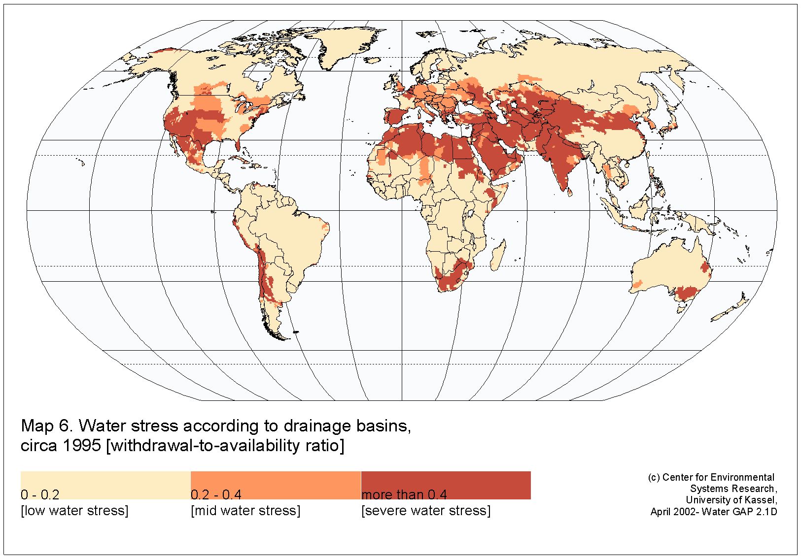
Using the concept of “water stress” we can compare the average condition of water resources around the world. In common usage, “water stress” is a measure of the amount of pressure put on water resources and aquatic ecosystems by the users of these resources, including the various municipalities, industries, power plants and agricultural users that line the world’s rivers. Here we use a conventional measure of water stress, the withdrawals-to-availability ratio*. This is the ratio of total annual water withdrawals divided by the estimated total water availability (equivalent to discharge). In principle, the higher the value of the ratio, the more intensively the waters in a river basin are used. Map 6 shows the withdrawals-to-availability ratio for the drainage basins of the world. Water stress is divided into “low”, “medium” and “high” classes according to commonly-used thresholds**. Nearly a quarter of the world’s terrestrial surface (excluding the ice caps) is in the severe stress category, including most of India, Northern China, Middle Asia, the Middle East, Northern and Southern Africa, parts of Southern Europe, Western Latin America, a large part of the Western United States, Northern Mexico, and a few drainage basins in Australia. In poorer countries a level of severe water stress indicates an intensive level of water use that likely causes the rapid degradation of water quality for downstream users, and absolute shortages during droughts. Also, in both developing and industrialized countries a level of severe water stress indicates strong competition for water resources during dry years between municipalities, industry and agriculture. Severe water stress areas occur mostly in arid areas of the world, as expected. However they also occur in the more humid drainage basins of the Don, Hudson, Severn, Thames, and most of Florida because of high water withdrawals.
(*) Compare, for example, Cosgrove, W. & Rijsberman F. (2000) World water vision: Making water everybody's business, Earthscan: London. Raskin, P., Gleick, P., Kirshen, P., Pontius, G. & Strzepek, K. (1997) Water Futures: Assessment of long-range patterns and problems, Comprehensive assessment of the freshwater resources of the world, Stockholm Environment Institute, Box 2142. S-103 14, Stockholm, Sweden.
(**) The thresholds of water stress are unknown and require scientific research. Here we use the thresholds from the references in (*).
Map 7. Area equipped for irrigation on a global grid
This is the percentage of area equipped for irrigation on a global grid (see Footnote 1) for around 1995.

Throughout history irrigation has been the dominant user of water resources. In 1995 it accounted for withdrawals of more than 2400 cubic kilometers globally, or 69 percent of total global withdrawals. Agricultural withdrawals are greater than the sum of industrial and domestic withdrawals in 37 percent of the area of the world, primarily in the developing part of the world. Using 1995 estimates, 3.1 billion people out of 5.6 billion lived in river basins where water for irrigation was the most important use*. The link between water and food is decisive because irrigation plays an essential role in world food production. Although irrigated land made up only 17 percent of the world’s cultivated land in the mid-1990s, 40 percent of the world’s food was produced here**. Map 7 depicts the areas with infrastructure needed for irrigation (“equipped for irrigation”). Although these areas are ready for irrigation, occasionally they may not be irrigated, as in the case when an unusually rainy growing season makes irrigation unnecessary. Today, irrigation is mainly practiced in three types of climate-zones. First of all, following a tradition of many centuries it continues to be used in the arid and semi-arid areas of the world, including coastal Peru, Egypt, West Pakistan, and Southwest Asia. Here agricultural production would be minimal without irrigation. Second, irrigation is used in regions with highly seasonal rainfall, for example with a Mediterranean climate as Central California and Southern Europe where irrigation makes cultivation in the summer possible. Also irrigation enables winter cultivation in parts of Asia affected by the monsoons. The third part of the world using irrigation are the fairly humid croplands in Russia, in western Europe and eastern United States where irrigation is used to boost yield in a typical year, and as a hedge against year-to-year swings in the amount of precipitation.
(*) These data were computed with the WaterGAP model and refer to the watershed area of the world where industrial water withdrawals are greater than either domestic or agricultural withdrawals.
(**) Rosegrant, M., Ringler, C. 2002. World water vision scenarios: consequences for food supply, demand, trade, and food security. In: Rijsberman, F. (ed.) World Water Scenarios and Analyses. Earthscan.
Map 8. Water withdrawals for irrigation on a global grid
This map shows the theoretical water requirements for irrigated crops, taking into account the climate of the climate normal period (1961-90), and that usually only a small percentage of an area is equipped for irrigation (Map 7). Data are given on a global grid (see Footnote 1). The units of mm indicate the volume of irrigation water (m3) required per unit of area of the grid cell (m2) used for irrigation. For example, if 10% of the area of a grid cell is irrigated, and irrigation water requirements are 10,000 m3 per hectare (1 ha = 10,000 m2) per year, then the annual water requirement in mm is: 0.10 x 10,000 m3/10,000 m2 x 1000 mm/1 m = 100 mm.

The amount of water needed by irrigated crops depends on many factors among which are the type of crop and cropping system, the irrigation approach and its level of technology, and the local climate and topography. On a per hectare and year basis, the water requirement for irrigation in arid areas is about 8000 cubic meters in Spain, and 10,000 in California. Obviously, where the efficiency of irrigation is lower, more water is required. For example in Egypt the average requirement is between 15,000 and 20,000 cubic meters*. Map 8 shows the water required for irrigation per unit area. To a certain extent the highest water withdrawals are located in areas with the highest density of irrigation projects (Map 7, area equipped for irrigation). This includes Pakistan and northern India, northern China, and the Central Valley of California. On the other hand, water requirements are also high in areas with a lower density of irrigation projects that are subject to intense evaporation because of local climate conditions such as much of India and China, Central Asia, much of the western United States, parts of western Latin America and Brazil, Southern Europe, the lower Don and Volga in Russia. In all these areas irrigation can be expected to be the dominant user of water.
(*) Llamas, M. 1997. Transboundary water resources in the Iberian Peninsula. In: Gleditsch, P. (ed.). 1997. Conflict and the environment. Kluwer: Dordrecht, The Netherlands. 335-353.
backMap 9. Water withdrawals for manufacturing industries according to drainage basins
This map shows the annual withdrawals for manufacturing estimated for 1995 on a drainage basin basis.

Water is one of the crucial raw ingredients of manufacturing. Its most important use in manufacturing is for cooling, as in the quenching of molten iron in the iron and steel industry. Its next most important use is as “process water” in which it makes up an essential part of the product stream. In the paper and pulp industry, for example, water is used for transporting ground wood and pulp from one process to another, for washing the pulp, for removing bark from pulp wood, and for cooking wood chips to remove lignin. In some industries, particularly canning, distilleries and other agro-industries, process water is literally a raw ingredient of the beverages and other canned products. Map 9 shows the world distribution of manufacturing water withdrawals per unit area. The highest levels of withdrawals follow the areas of highest population density, including Pakistan and northern and southern India, much of eastern China, the eastern two-thirds of the United States and parts of Canada, the northwestern, southwestern and eastern parts of Latin America, much of Europe and Central Russia, the Nile basin in Africa, and the Middle East. The waterways in many of these areas are under severe water stress (see Map 6 on water stress). In a strong competition for scarce water resources manufacturers normally have the economic advantage and can drive out irrigation water users.
backMap 10. Consumptive water use for cooling in thermal power plants

Producing electricity at thermal power plants requires substantial amounts of water during every stage of the energy cycle from mineral extraction to delivery of the fuel to the power plants. But by far the greatest need for water comes from the cooling of turbines in the power plant. The amount of water required depends on the type and size of power plant, and especially on the kind of cooling. The two main types are “once-through cooling”, in which water is used to cool the turbines and then discharged directly back to a waterway or pond, and “tower cooling” in which the turbines are cooled and the hot water is sent to a cooling tower, reused several times, and eventually discharged from the plant. One of the advantages of tower cooling is that water is discharged back to waterways at a much cooler temperatures, thereby protecting aquatic ecosystems and downstream water uses. Another advantage is that it allows the recycling of water within the power plant, and this means that tower cooling requires less than three percent of the water withdrawals of once-through cooling (per unit energy produced). Although tower cooling requires much lower withdrawals, it consumes twice as much water per unit energy as once-through cooling because much more water is evaporated in the cooling towers. Map 10 shows the location and water consumption of thermal power plants. Because they deliver electricity for the population and its economic activity, power plants tend to be situated near population centers; because of their large water requirements, they also are usually sited near large waterways or other bodies of water. Map 10 also vividly shows the intensity of water consumed for power production in Europe and North America as compared to the rest of the world.
backMap 11. Water withdrawals for cooling in thermal power plants according to drainage basins

Map 11 shows the volume of water withdrawn by thermal power plants per unit area. These withdrawals are highest in northern and central India, the eastern half of China, Japan, Korea, through much of North America, parts of Latin America, through much of Europe, and in the Nile Basin in Africa. Because thermal power plants are reliant on large sources of water, the areas of highest withdrawals tend to be more geographically concentrated than manufacturing industries (see Map 9), or households (see Map 12). Nevertheless, most of the water withdrawn by thermal power plants is used and then returned to waterways without a major degradation of quality (except for thermal pollution caused by once-through-cooling). Hence their overall average impacts on downstream users are often smaller than that of manufacturers or municipalities which withdraw water, use it, and discharge it back to waterways with degraded quality.
backMap 12. Water withdrawals for households according to drainage basins
This map shows the annual withdrawals for household and commercial uses estimated for 1995 on a drainage basin basis.

Cities require large volumes of water for their existence and much of this is used in households to cover the basic personal needs of urban dwellers. As can be imagined, the profiles of household water use in developing and industrialized countries are quite different. In developing countries they include water for drinking, cooking and bathing. In addition to these basic needs, the current Western lifestyle requires considerable extra amounts of water for washing clothes, dishes and cars. Many industrialized countries also have very substantial outdoor water demands for watering lawns and gardens, and for maintaining swimming pools. In arid climates outdoor water uses can make up a huge fraction of total water use. But on the average the largest fraction of water used in industrialized countries is for toilet flushing, followed by clothes washing, showering and faucet use. The differences in personal requirements also lead to huge differences in the volumes of water used between countries – the average North American uses about 400 liters per person per day while the typical sub-Saharan African, around 10 to 20 liters per day*. Map 12 shows the water withdrawals for households per unit area. The data in this map also includes water withdrawals for supplying the needs of commercial businesses in cities and rural areas. These needs are much the same as household requirements – water use for toilets, kitchens, and sinks – but include additional uses for process water, large restaurant kitchens, and sometimes decorative landscaping. Household plus commercial uses account for approximately 10 percent of the total withdrawals of water in the world. Hence the most essential requirements for water – drinking, cooking, and hygiene – are covered by a relatively small fraction of the world’s water withdrawals. Map 12 shows that the needs for households are more spread out around the world than water uses for other purposes. This is expected since wherever people live, they require basic water services. Higher water withdrawals per unit area are found through much of Europe, South and Northeast Africa, large parts of Latin America and much of North America. In some places such as India, Pakistan, China, and Northeast Africa the household use per person is lower than in industrialized countries, but the density of people is higher. Hence the water withdrawals per unit area are of the same order of magnitude as in industrialized countries.
(*) Rijsberman, F. (ed.) 2002. World water scenarios and analyses. Earthscan: London.
backMap 13. Internal renewable water resources generated within a country on a per capita basis, circa 1995 [m³/cap/annum]
The map shows the per capita total internal renewable water availability by country. This is the fraction of the country’s water resources that is generated within the country. Units are m³ per capita and year.

The total internal renewable water resource is defined as the average long-term annual discharge (1961-1990) generated from endogenous precipitation, taking into account evaporation losses from lakes and wetlands, even if this might be dependent on the inflow from other countries (this definition differs from that of the WRI and may lead to negative values). Here the total internal renewable water availability is shown in m³ per capita and year. Generally, the semiarid and arid areas of the globe have low internal renewable water availabilities. However, the internal availabilities are compared as mean values for the entire country, although high regional variability within the country is possible (e.g. Australia). Furthermore the total available internal resources are divided by the total population of the country. Consequently, countries with low population have higher values compared to countries with the same internal renewable water availability but higher population.
backMap 14. Percentage of area under severe water stress based on cell-level computations by country
This is the fraction of the country’s water resources that is generated within the country. Units are m³ per capita and year.

This map is based on cell-level computations (0.5°x 0.5°) of the WATERGAP model. It is assumed that values of withdrawal-to-availability ratio larger than 0.4 represent severe water stress. Cell areas within a country with severe water stress have been summed up to determine the percentage in relation to the entire country area. Countries with high percentages of severe water stress (more than 50 % of country area) can be identified in Europe (Belgium Spain, Bulgaria), in the Southern Mediterranean area (Libya), in the Near and Middle East (Iran, Turkmenistan, Uzbekistan, Pakistan), and the Arabian peninsula.
backMap 15. Change in water stress according to drainage basin
This map shows annual total water withdrawals estimated for 1995 on a drainage basin basis.

The changes in water withdrawals have been calculated as a ratio of the total withdrawals for 1970 and 1995. The total withdrawal is computed as the sum of withdrawals from the domestic, industrial, livestock, and irrigation sectors. To determine the 1970’s domestic and industrial withdrawals, historical data of Shiklomanov (2000) based on 26 world regions have been used, whereas the 1970 irrigation values were calculated with FAO historical data (FAO 2001). Due to the fact that the withdrawal from livestock is small compared to the other sectors, this value remains constant for the whole period 1970-1995. Small changes or a decrease of total water withdrawal (less than 5%) can be observed in basins in the US East-coast, in Northern Europe and Northern Canada, as well as in central parts of Australia and West Egypt. High increases (larger than 75%) have been computed for the lower Amur basin, the Lake Aral area and Caspian Sea, Eastern Mongolia, Northern Libya, the Indus basin, the lower Ganges basin, as well as the Namibian part of the Oranje River.
backMap 16. Area equipped for irrigation vs total arable land by country
This map shows the area equipped for irrigation vs total arable land by country. The total arable land was taken from World Resources Institute (1998).

This map shows the area equipped for irrigation in relation to the total arable land per country in percentage. The total arable land data provided by WRI (1998). High percentages (more than 50%) can be observed in countries of Eastern Asia, Middle East, Madagascar, as well as Chile, Guyana, and Surinam.
backMap 17. Increase in irrigation requirement in a typical dry year compared to the long-term average on a global grid
The map shows the irrigation requirements in a typical dry year compared to the long-term average (1901-1995).

The increase in irrigation requirements for a typical dry year compared to the long-term average shows generally an increase of the irrigation requirements. This is due to the fact that in a typical dry year the water availability decreases (e.g. less precipitation occurs), thus the water demand for irrigation increases. The highest increase in water demand are observed in Southern Brazil, the costal parts of Peru, Ecuador, Columbia, the eastern part of Manchuria in China and the area around the northern border with Burma (Northern Mekong basin), as well as Japan. In general, the larger the long-term average irrigation requirement is, the lower the percentage increase in the cell specific 1-in-10 dry year will be and vice versa. This means that in regions with high long-term average irrigation requirements, where essentially all the water necessary for crop growth is be provided by irrigation, the increase of irrigation requirements in a typical dry year is low (see also Döll 2002)*.
(*) See also Döll, P. (2002): Impact of climate change and variability on irrigation requirements: a global perspective. Climatic Change (in print).
backMap 18. Water withdrawals for irrigation as ratio of the total withdrawals according to drainage basins
The map shows water withdrawals for irrigation as a ratio of the total withdrawals according to drainage basins in percentage for the present situation (circa 1995).

In this map the ratio of water withdrawals for irrigation to the total withdrawals in drainage basins is shown. Generally, the basins with a high fraction of areas equipped for irrigation also claim high withdrawals. These basins are mainly located in arid to semi-arid areas of the world, like Northern Africa and Southwest Asia.
backMap 19. Combined map showing the drainage basins under medium or high water stress and the water use sector which claims the highest fraction of withdrawals in these drainage basins

In relation to map 18, map 19 shows the drainage basins with medium to high water stress and the water use sector which claims the highest fraction. The spatial distribution shown in map 18 is repeated in this map for the irrigation fraction. Generally, the irrigation sector dominates the water withdrawals, followed by industry, domestic, and livestock. However, industrial withdrawals are dominant in Central Europe, the East coast of the USA, the great lakes region in northeastern USA, Japan, and Korea, as well as in the Ukraine and the southwestern part of the Russian Federation.
backMap 20. Water use in a certain country’s part of a transboundary river basin as ratio of total water use in the basin

Map 20a - Proportions of the single country’s part of selected transboundary basin

The water use in selected transboundary basins has been subdivided into the respective countries fractions. Map 20 shows the largest 24 transboundary basins. The accompanying map 20a quantifies the proportions of the single country’s part of selected transboundary basin. Furthermore a table was generated showing the country’s fractions of the largest transboundary river basins. Due to the fact that the calculations have been computed on a 0.5° grid cell level, boundary cells have been attributed to the country covering the major part of the cell. Therefore, some countries, which are part of a transboundary basin, but with a very small proportion of the entire basin, do not appear (e.g. Poland, Italy and Albania for the Danube basin with fractions lower than 0.1 % of the total basin extent (compare WOLF et al 1999)*). Further the map shows also drainage basins, that have only periodically discharge as for example the Area Cyrenaica (Libya; Egypt)
(*)Wolf, A. Natharius, J. Danielson, J. Ward, B. & J. Pender (1999): International river basins of the world. Water Resources Development, Vol. 15, No. 4, 387-427.
backMap 21. Coefficient of variation of annual discharge according to drainage basins

The coefficient of variation of the annual discharge has been computed according to drainage basins. The map shows the percentage of variation in relation to the long term average runoff (1961-1990). Generally, the semiarid and arid regions with low runoff show a high variance in the discharges. Especially the Sudan-Sahel-Sahara area, southern parts of Africa, Australia, Middle East countries, as well as eastern parts of Brazil and Northern Mexico show high variances in discharges.
backMap 22. Annual runoff in the 1-in-10 dry year as a ratio of the long-term average annual runoff on a global grid

To show the impact of the interannual variability on water availability, the runoff in the cell-specific 1-in-10 dry year is compared to the long-term average total cell runoff for the time period 1961 to 1990. This means that in 90 % of the months the runoff is higher than in the 1-in-10 dry year. The interannual runoff variability is highest in those regions of the globe with a low average cell runoff. The 1-in-10 dry year runoff provides a stronger spatial discrimination of water resources situation than the long- term average runoff and represents the situation in a potential crisis year. Therefore it is a useful additional indicator of water availability. The map show the percentage of the 1-in-10 dry year in relation to the average annual runoff (Döll et al. 2002)*.
(*)Döll, P., Kaspar, F. & B. Lehner (2002): A global hydrological model for deriving water availability indicators: model tuning and validation (submitted to Journal of Hydrology).
backMap 23. Water stress in regions around selected mega cities

The global map shows the water stress in three classes as ratio of withdrawals-to-availability (low stress 0 – 0.2, medium stress 0.2 – 0.4, and severe stress > 0.4) and the location of the twenty largest mega cities (UNEP 2002). The largest mega cities are additionally shown to highlight the water stress in their surrounding regions. Each circle has a radius of 200 km. In most cases there is a strong correlation between areas with severe water stress and mega cities as major water consumers. For mega cities located in regions which are already under water stress a further growth is restricted due to a limited water availability. However, this is not the case in Lagos, Buenos Aires, or Sao Paulo, where basins do not show severe water stress. To avoid the overexploitation of the natural river basins and to provide enough water for industrial and domestic use, most of the mega cities import water from surrounding basins.
backMap 24. Dependence of the countries’ water resources on inflow from neighbouring countries: inflow as a ratio of total water availability (internal renewable water resources plus inflow)

This map show the dependence of a country’s water resources on inflowing water from neighbouring countries in percentage (inflow over internal plus inflow). High dependence is observed in Central and Southern Africa, as well as Middle East and East Asia.
backReferences
UNEP (2002): Global Environment Outlook 3. Past present and future perspectives. Earthscan Publications, London, Sterling.
Döll, P., Kaspar, F. & B. Lehner (2002): A calibrated global hydrological model for deriving water availability indicators (submitted to Journal of Hydrology).
Döll, P. (2002): Impact of climate change and variability on irrigation requirements: a global perspective. Climatic Change (in print).
Shiklomanov, I. (2000): World water resources and water use. Present assessment and outlook for 2025. In: Rijsberman, F.R. (ed.) World Water Scenarious: Analysing Global Water Resources and Use, Earthscan Publications, London.
Wolf, A. Natharius, J. Danielson, J. Ward, B. & J. Pender (1999): International river basins of the world. Water Resources Development Vol. 15, No.4, 387-427.
FAO (2001) (United Nations Food and Agriculture Organization): historical data of irrigated areas. In: http://www.fao.org.